Predicting the Over/Under in the EPL Using Machine Learning

5 min readJul 31, 2020

Introduction

We will be looking at Premier League matches and predicting whether the game will go over or under 2.5 goals. We chose football because it is for the majority of the time a fairly low-scoring game, with the English Premier League, being one of the lowest scoring leagues, averaging just above 2.5 goals. Another reason for choosing the EPL was for its competitiveness: teams often compete for the Champions and Europa League qualification as well as to stay out of the relegation zone, well into the end of the season.

Data

To build our predictive models we used data from the 2014 season to the 2018 season. In order to obtain more predictive features we combined two different datasets for each season. One containing team and match statistics and the other containing betting data.

Baseline

In order to establish a baseline we simply took the majority class of the two outcomes; 1 being over 2.5 and 0 being under 2.5. As can be seen the amount of games that go over and under 2.5 goals are fairly even. What this means is that our basic model is basically predicting every game will go over 2.5 goals and has an accuracy of 51.8%.

Approach

We will be using 3 different models to predict whether an individual match will have either less than or greater than 2.5 goals. Since we are dealing with a binary target, this is a classification problem by nature and thus will be using classification algorithms. As the sole evaluation metric we will be using accuracy which is the number of correct predictions divided by the number of total predictions.

Models

Logistic Regression: A linear model used for predicting a categorical target. The more independent variables it has the more it is prone to over-fitting. This is the simplest model of the three.

Random Forest Classifier: An algorithmic model that consists of a multitude of decision trees. Each individual tree predicts a class and the class with the most votes becomes the model’s prediction. Using this process makes it less likely to become over-fitted to the training set data.

XGBoost Classifier: A model which uses Gradient Boosting, which builds on the previous model’s weakness to produce a much stronger model at the end. It is slightly similar to the Random Forest Classifier in that it is an ensemble method but the major difference is that it builds trees sequentially and instead of combining trees at the very end it combines them in the process.

Results

We began by first creating the train, validation, and test sets with features that were deemed important and then running every single model. Initially we saw that the highest of the 3 models (Random Forest Classifier) was about 56%, however the feature selection was negatively affecting the accuracy predictions.

To improve the accuracy scores, we chose features which had a positive impact on the models; the XGBoost Classifier model ended up with the best accuracy score of 60%. To put the results in perspective here is a confusion matrix showing the testing dataset. It shows all of the predictions that were made and which ones were correct and incorrect.

Conclusion

We were successful in creating a model that would beat the baseline model. In order to achieve such a high accuracy score we had to first select the best features and then fine tune the parameters in XGBoost Classifier model.

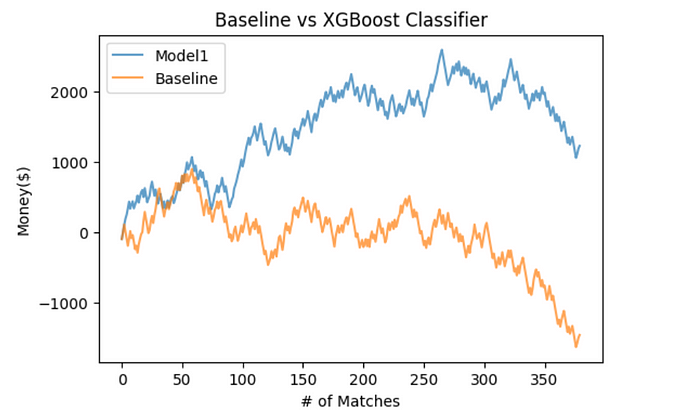
Now the real question is how profitable is this model? To find out, we did some more analysis on our testing data to see how it would match up against actual betting odds. To do this we simply bet the predicted outcome of every single game in the 2018 season(380) and compared it to the major class Baseline model that had a 53% accuracy score. At the end of the season the Baseline total profit loss was -$1,462 and the XGBoost Classifier model achieved a profit of $1,222, a significant difference of about $2,000 with an accuracy improvement of 7% . One thing worth noting is that in the last quarter of the season, both models pictured in the graph below started to have a negative trend. This may be due to the fact that as the the season progresses the sports betting market becomes more efficient because of more data availability, effectively making it harder to beat the bookmakers.

However, it should be noted that 3 seasons were used to train the model, 1 year for validation, and 1 year for testing. Both the validation and testing accuracy scores were above 58%, but before using this model for future seasons, one would have to back-test using more seasons in order to establish more consistency and eliminate any possibility of over-fitting. Additionally, we could improve the features with better data and with further hyperparameter tuning. Also, more realistically we would not be betting on every single game and instead be more selective on the matches we choose to bet on. This being said, our model was a success and it can serve as a building block to further improve similar models.